Applying MLOps to Industrial Water Pump Anomaly Detection
Introduction: Setting the Stage
In an industrial environment, readings are continuously generated by water pumps. Every minute, there’s more data to process, and simply having that data doesn’t make it useful on its own.
Training a machine learning model is usually the first thing people think about. In an MLOps setup, getting that model to work reliably with real-world data is a different problem.
The real challenge is spotting unusual operating conditions early. When sensor data is monitored manually, changes in pump behaviour can be easy to miss, especially as the volume of data grows. If those changes aren’t noticed in time, a developing equipment issue may be harder to catch before it becomes a larger problem. That’s the problem we wanted to address with our water pump anomaly detection pipeline.
This blog looks at how MLOps can be used to address this problem by connecting the different stages of the machine learning lifecycle into one automated pipeline. The goal wasn’t to predict failures directly. Instead, we focused on finding unusual patterns in the sensor data that might point to unexpected pump behaviour.
But detecting an anomaly was only one part of the problem. This is where MLOps comes in. The sensor data still has to move through ingestion, validation, transformation, model training, deployment, and monitoring. We wanted these steps to work together so the pipeline could be run repeatedly without someone manually starting each step.
The Challenge: More Than Training a Model
A basic ML workflow can be quite simple. Run a script. Check the data. Train the model. Start the API. That’s fine while you’re experimenting.
It becomes harder when the same process needs to run regularly. If one script fails, someone must notice. If new data arrives, it needs to be picked up without being processed twice. If a new model is trained, there needs to be a clear record of which version it is.
Then there’s production.
The model can be running perfectly from an infrastructure point of view while the incoming data has started to change. The API may still return predictions. The dashboards may still be up. Nothing looks obviously broken. But the predictions may no longer mean the same thing. For an industrial system, that’s something worth catching early.
Catching that kind of change early isn’t something a single script or a one-off check can do. It depends on how the different stages, ingestion, validation, training, deployment, and monitoring, are connected, and on someone actively watching each one. That’s the structure behind the pipeline described next.
Inside the Pipeline
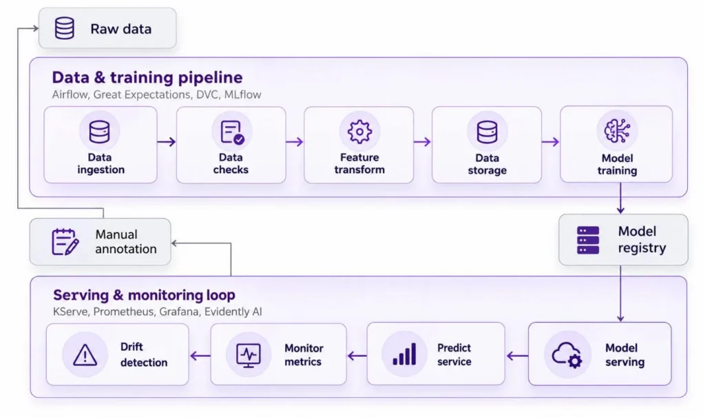
The pipeline brings together the data, ML and operational parts of the workflow.
In an MLOps pipeline, it isn’t always clear which part is handled by whom, especially when multiple teams are involved. In this setup, the ML Team (Development) handles the model and data-related work, while the Ops & Automation Team focuses on orchestration, deployment, monitoring, and automation. The table below shows how these responsibilities are divided across each stage of the pipeline.
| Pipeline Stage | Technology | ML Team (Development) | Ops & Automation Team |
|---|---|---|---|
|
Data Ingestion |
Airflow, Python |
Define data requirements and pipeline logic. |
Automate data ingestion and orchestrate workflows. |
|
Data Validation |
Great Expectations |
Define validation rules and quality thresholds. |
Implement validation checks and failure handling. |
|
Model Training |
Isolation Forest, MLflow |
Build, train, track, and register models. |
Automate training workflows and maintain MLflow infrastructure. |
|
CI/CD & Deployment |
GitLab, Docker, Kubernetes, KServe |
Validate model behaviour before release. |
Build containers, manage CI/CD, and deploy scalable inference services. |
|
Monitoring |
Prometheus, Grafana |
Define monitoring metrics, thresholds, and retraining criteria. |
Configure dashboards, alerts, and operational monitoring. |
|
Drift Management |
Evidently AI |
Review drift reports and decide retraining strategy. |
Generate drift reports, trigger alerts, and automate pipeline re-execution. |
The pipeline isn’t one large script doing everything. The different parts can be managed and understood separately.
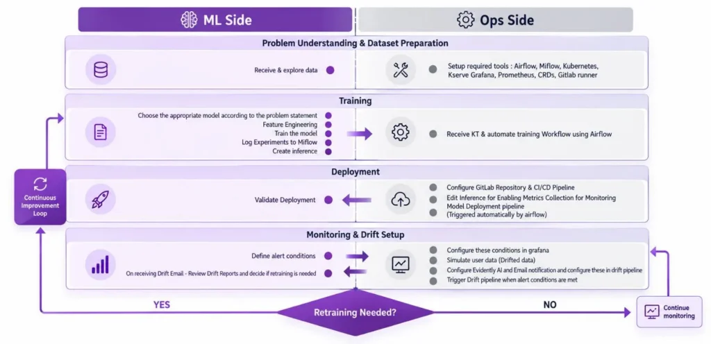
Alongside the responsibility table above, we also put together a visual timeline of the pipeline, shown below. The timeline shows how the work is divided between the ML Side and the Ops Side across each stage of the MLOps pipeline. It isn’t always clear from the pipeline alone which team handles a task or when the handoff happens, so this view makes the sequence and ownership easier to follow. Read the below chart (Fig: MLOps Lifecycle & Continuous Improvement Framework), from top to bottom: the purple side represents ML activities, the green side represents Ops activities, and the orange arrows show handoffs between the two teams. The loop at the bottom shows what happens after monitoring, depending on whether retraining is needed.
Making the Pipeline Run on Its Own
One of the first problems we had to solve was orchestration.
Running a few scripts manually isn’t difficult. Remembering to run them in the right order every time is. We use Apache Airflow to manage this workflow.
Airflow handles the sequence from data ingestion through validation, transformation and training. It also gives us visibility into individual tasks, so when something fails, we don’t have to guess which part of the process went wrong.
This is useful for another reason.
The workflow can be reused. Instead of someone sitting down and manually starting each script whenever new data needs to be processed, the pipeline has a defined flow that can be executed again.
Each tool has a separate role. Airflow manages the workflow, GitLab handles CI/CD, Docker packages the application, and Kubernetes with KServe handles serving.
Catching Bad Data Early
A model can only work with the data it receives.
If the incoming data is missing a column or contains an unexpected data type, there’s no good reason to let it continue through the rest of the pipeline. We use Great Expectations for this first check.
Before the data moves ahead, we make sure the columns and values are in the format we expect. If it doesn’t pass, the pipeline stops. That’s useful because the problem is caught before it reaches training.
This is where shift-left validation helps. The check happens near the beginning, when the problem is still small and easier to investigate.
It’s a simple idea. Check the data before depending on it.
Preparing the Data and Training the Model
Once the data passes validation, it moves through the transformation stage.
The sensor values are prepared and scaled before training. The processed data is then used by the anomaly detection model.
We use Isolation Forest (algorithm for anomaly detection) for this catching bad entry because the dataset doesn’t contain labelled anomaly outcomes. There isn’t a reliable column telling us which individual observations represent an actual equipment failure.
That changes the modelling approach. Instead of training a supervised classifier against known failure labels, Isolation Forest looks for observations that appear unusual compared with the rest of the data.
MLflow keeps track of the training runs, including parameters, metrics, artifacts and model versions. That gives us a record of how a particular model was created.
It also solves a very practical problem. If someone asks which model is currently being used, we shouldn’t have to search through old files to figure it out.
Once the model is successfully registered, the workflow can move towards deployment.
Moving From a Model File to a Running Service
Having a trained model doesn’t mean the work is finished.
The model still needs a way to receive sensor data and return predictions. It also needs to move through a repeatable deployment process rather than being copied and started manually.
After the model is registered, Airflow reaches the deployment step and triggers GitLab. The application is packaged into a Docker image and passed on to the Kubernetes environment. KServe then takes care of running the model there.
After that, the model is ready to receive the pump readings and identify whether a reading looks normal or unusual.
Once the inference service is available, incoming sensor readings can be sent to it and scored by the model.
What Happens After Deployment?
To show how the pipeline behaves once it’s live, without waiting around for real drift to occur naturally, we built a demonstration environment that mimics a production deployment. We used historical pump data and replaying it to simulate a live stream. The dataset contains around 109,440 records covering roughly 75 days of sensor readings. Part of which is used for training, remaining unseen data is sent in batches of 500 with a short delay between batches to see how the model behaves.
We trained the model using summer data. Later, we introduced winter data during the inference stage.
That’s where things became interesting.
The sensor readings in winter don’t follow the same patterns as the summer readings. When those new readings reach the model, some of them look unusual compared with the patterns it learned during training.
The inference service continues running. Predictions still come back. But the anomaly rate starts changing. This is where monitoring becomes important.
Prometheus collects metrics from the inference service, including prediction counts, anomaly counts, latency, inference throughput and rolling anomaly rate.
Grafana gives us a way to see those changes over time.
A single anomalous prediction doesn’t tell us much. A sustained increase in the anomaly rate is much more useful.
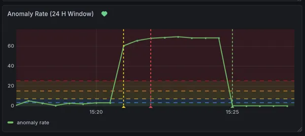
In our setup, a rolling anomaly rate of 15% is used as the alert threshold. When the rate crosses that threshold, we don’t immediately assume that the model has failed.
We investigate first.
Watching the Data Change
That change can lead to more observations being flagged as anomalous.
The API can still be healthy. The predictions can still be coming back. The important change is in the data and in the behaviour of the predictions. This is where we look beyond the threshold itself.
If the anomaly rate crosses 15%, we can use Prometheus to track what happens next. Is the rate continuing to increase? Has it started to come down? Or is it staying around the same level? The graph below shows an example of how the anomaly rate changes over time after crossing the 15% threshold.
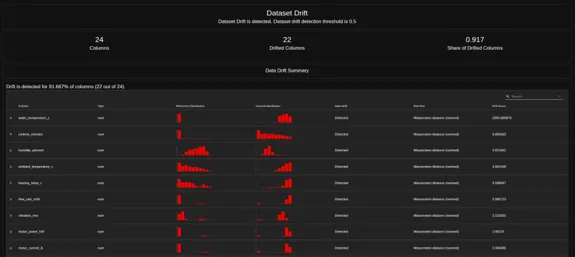
Evidently can then be used to examine the change in the incoming data and generate a drift report. This gives the team another view of what changed before deciding whether retraining is needed. The report below shows the detected changes across the incoming sensor features and gives the team another view of what changed before deciding whether retraining is needed.
That trend gives us more information than the alert alone.
For example, an anomaly rate that crosses 15% and keeps increasing needs a different level of attention from one that briefly crosses the threshold and then returns to normal. We can also require the rate to remain above the threshold for a defined period before treating it as a condition that needs further investigation.
The same information can be included in an automated monitoring report.
Instead of simply saying that the 15% threshold was crossed, the report can show when it happened, how long the anomaly rate stayed above the threshold, and whether the rate was increasing, decreasing or remaining relatively stable.
That gives the engineering team a clearer starting point for investigation. The investigation then helps answer the next question.
Is this a genuine change in operating conditions, or is there a problem with the data or the model?
In our example, the change in sensor behaviour is linked to the difference between the summer data used for training and the winter data being processed later. If the investigation shows that the new operating conditions are valid and are expected to continue, the next step can be retraining the model with representative data.
The updated data can then go through the pipeline again, from validation and transformation through training and model registration, before the updated model is moved towards deployment.
Retraining isn’t triggered simply because an alert appeared. The alert starts the investigation. The investigation provides the reason for the next step.
Why the Different Pieces Matter
It would be easy to look at this setup and see a long list of tools.
Airflow. Great Expectations. MLflow. GitLab. Docker. Kubernetes. KServe. Prometheus. Grafana. But the tools aren’t the main point.
The useful part comes from connecting these pieces.
Without orchestration, there are scripts.
Without validation, there is a risk of bad data moving forward.
Without tracking, it becomes harder to understand where a production model came from.
Without monitoring, problems can sit unnoticed.
MLOps brings those concerns into the same workflow.
Conclusion: Keeping the Model Running
A trained model is only one part of a production ML system.
For an industrial use case like water pump anomaly detection, the surrounding process matters just as much. Data needs to arrive properly. Bad inputs need to be caught early. Training runs need to be traceable. Deployment needs to be repeatable. And once the model is running, there needs to be enough visibility to understand what is happening. That’s what we were trying to solve with this pipeline.
Not every problem needs another tool. Not every change in production data means a model needs to be retrained. And not every part of an ML workflow needs to be complicated.
At MosChip, that’s an important part of how we look at machine learning in production. Making sure the system around it can keep running, be monitored, and be understood when something changes is the part that makes it useful beyond a development environment.
The question isn’t only whether the model works. It’s also largely whether we can keep it working. To know more about our MLOps offerings, get in touch with our team today!
FAQs
The dataset doesn’t contain labelled failure or anomaly outcomes. Because of that, a supervised classification approach isn’t a good fit. Isolation Forest works without labelled anomalies and identifies sensor readings that look unusual compared with the rest of the data.
Yes. Prometheus can track the anomaly rate over time and compare the current value with previous time windows. This makes it possible to see whether the rate is continuing to increase, starting to fall, or remaining relatively stable after crossing the threshold.
This can also be used for automated reporting. For example, if the anomaly rate remains above the threshold for a defined period, an automated report can include the current anomaly rate, how long the threshold has been exceeded, and whether the rate is trending upward, downward, or staying stable.
That gives the team more context than a simple threshold alert and can help decide whether the change needs further investigation.
Yes. That’s one of the reasons the workflow is orchestrated rather than handled through individual manual scripts.
Once the investigation shows that retraining is appropriate, the updated data can go through the same validation, transformation, training and registration flow. The resulting model can then move through the deployment process again.
That change is useful information too. If the anomaly rate crosses the threshold and later returns below it, the team can look at the duration and trend of the event rather than treating the threshold crossing as a permanent failure. This is one reason tracking the rate over time is more useful than looking at a single alert in isolation.
An alert tells us that something changed. It doesn’t tell us why. The increase could be related to a genuine change in operating conditions, a change in the sensor data, or a problem that needs to be investigated first. Retraining immediately could make the model learn from a temporary or incorrect condition. That’s why the alert starts the investigation rather than automatically replacing the model.
The investigation needs to establish whether the new data represents a valid and continuing operating condition.
In our example, the winter readings differ from the summer data used during training. If those winter conditions are genuine and expected to continue, they can provide useful data for a future training cycle.
The decision should be based on the behaviour of the equipment and the quality of the new data, not just on the fact that an alert was triggered.
Share this article on:
-
 View other Blogs
Bhanu Prakash Yakkaluri is an RTL Design Manager with over 15 years of experience in ASIC/SoC design and implementation. He has worked on complex HPC processor-based SoCs, including designs based on Arm Neoverse V2. He has contributed across the complete frontend design flow, from micro-architecture to RTL design and functional verification. He has delivered multiple successful tapeouts across technology nodes ranging from 180nm to 5nm. His expertise includes clock and reset architecture, SoC integration, multi-clock domain design, and CDC/RDC analysis. He is proficient in synthesizable RTL design, netlist verification, and automation using Perl scripting. He has strong knowledge of high-speed industry-standard protocols such as IEEE 802.3ae, IEEE 802.11 MAC, and eUSB, AMBA Bus Architectures